A Velox Primer, Part 3

At the end of the previous article, we were halfway through running our first distributed query:

SELECT l_partkey, count(*) FROM lineitem GROUP BY l_partkey;

We discussed how a query starts, how tasks are set up, and the interactions between plans, operators, and drivers. We have also presented how the first stage of the query is executed, from table scan to partitioned output - or the producer side of the shuffle.  

In this article, we will discuss the second query stage, or the consumer side of the shuffle.

Shuffle Consumer

As presented in the previous post, on the first query stage each worker reads the table, then produces a series of information packets (SerializedPages) intended for different workers of stage 2. In our example, the lineitem table has no particular physical partitioning or clustering key. This means that any row of the table can have any value of l_partkey in any of the files forming the table. So in order to group data based on l_partkey, we first need to make sure that rows containing the same values for l_partkey are processed by the same worker – the data shuffle at the end of stage 1.

The overall query structure is as follows:

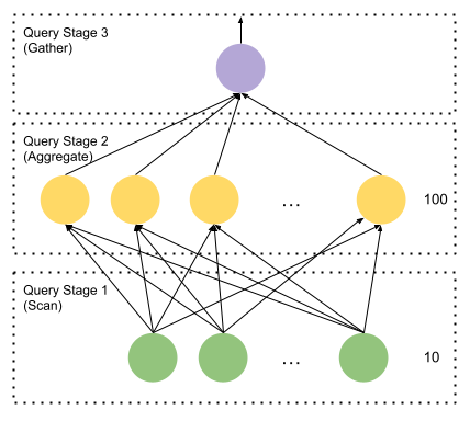
The query coordinator distributes table scan splits to stage 1 workers in no particular order. The workers process these and, as a side effect, fill destination buffers that will be consumed by stage 2 workers. Assuming there are 100 stage 2 workers, every stage 1 Driver has its own PartitionedOutput which has 100 destinations. When the buffered serializations grow large enough, these are handed off to the worker's OutputBufferManager. 

Now let’s focus on the stage 2 query fragment. Each stage 2 worker has the following plan fragment: PartitionedOutput over Aggregation over LocalExchange over Exchange.  

Each stage 2 Task corresponds to one destination in the OutputBufferManager of each stage 1 worker. The first stage 2 Tasks fetches destination zero from all the stage 1 Tasks. The second stage 2 fetches destination 1 from the first stage Tasks and so on.  Everybody talks to everybody else. The shuffle proceeds without any central coordination.

But let's zoom in to what actually happens at the start of stage 2.

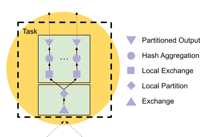
The plan has a LocalExchange node after the Exchange. This becomes two pipelines: Exchange and LocalPartition on one side, and LocalExchange, HashAggregation, and PartitionedOutput on the other side. 

The Velox Task is intended to be multithreaded, with typically 5 to 30 Drivers. There can be hundreds of Tasks per stage, thus amounting to thousands of threads per stage. So, each of the 100 second stage workers is consuming 1/100 of the total output of the first stage. But it is doing this in a multithreaded manner, with many threads consuming from the ExchangeSource. We will explain this later.

In order to execute a multithreaded group by, we can either have a thread-safe hash table or we can partition the data in n disjoint streams, and then proceed aggregating each stream on its own thread. On a CPU, we almost always prefer to have threads working on their own memory, so data will be locally partitioned based on l_partkey using a local exchange. CPUs have complex cache coherence protocols to give observers a consistent ordered view of memory, so reconciliation after many cores have written the same cache line is both mandatory and expensive. Strict memory-to-thread affinity is what makes multicore scalability work. 

LocalPartition and LocalExchange

To create efficient and independent memory access patterns, the second stage reshuffles the data using a local exchange. In concept, this is like the remote exchange between tasks, but is scoped inside the Task. The producer side (LocalPartition) calculates a hash on the partitioning column l_partkey, and divides this into one destination per Driver in the consumer pipeline. The consumer pipeline has a source operator LocalExchange that reads from the queue filled by LocalPartition. See LocalPartition.h for details. Also see the code in Task.cpp for setting up the queues between local exchange producers and consumers.

While remote shuffles work with serialized data, local exchanges pass in-memory vectors between threads. This is also the first time we encounter the notion of using columnar encodings to accelerate vectorized execution. Velox became known by its extensive use of such techniques, which we call compressed execution. In this instance, we use dictionaries to slice vectors across multiple destinations – we will discuss it next.

Dictionary Magic

Query execution often requires changes to the cardinality (number of rows in a result) of the data. This is essentially what filters and joins do – they either reduce the cardinality of the data, e.g., filters or selective joins, or increase the cardinality of the data, e.g. joins with multiple key matches.

Repartitioning in LocalPartition assigns a destination to each row of the input based on the partitioning key. It then makes a vector for each destination with just the rows for that destination. Suppose rows 2, 8 and 100 of the current input hash to 1. Then the vector for destination 1 would only have rows 2, 8 and 100 from the original input. We could make a vector of three rows by copying the data. Instead, we save the copy by wrapping each column of the original input in a DictionaryVector with length 3 and indices 2, 8 and 100. This is much more efficient than copying, especially for wide and nested data.

Later on, the LocalExchange consumer thread running destination 1 will see a DictionaryVector of 3 rows. When this is accessed by the HashAggregation Operator, the aggregation sees a dictionary and will then take the indirection and will access for row 0 the value at 2 in the base (inner) vector, for row 1 the value at 8, and so forth. The consumer for destination 0 does the exact same thing but will access, for example, rows 4, 9 and 50.

The base of the dictionaries is the same on all the consumer threads. Each consumer thread just looks at a different subset. The cores read the same cache lines, but because the base is not written to (read-only), there is no cache-coherence overhead. 

To summarize, a DictionaryVector<T> is a wrapper around any vector of T. The DictionaryVector specifies indices, which give indices into the base vector. Dictionary encoding is typically used when there are few distinct values in a column. Take the strings “experiment” and “baseline”. If a column only has these values, it is far more efficient to represent it as a vector with “experiment” at 0 and “baseline” at 1, and a DictionaryVector that has, say, 1000 elements, where these are either the index 0 or 1.  

Besides this, DictionaryVectors can also be used to denote a subset or a reordering of elements of the base. Because all places that accept vectors also accept DictionaryVectors, the DictionaryVector becomes the universal way of representing selection. This is a central precept of Velox and other modern vectorized engines. We will often come across this concept.

Aggregation and Pipeline Barrier

We have now arrived at the second pipeline of stage 2. It begins with LocalExchange, which then feeds into HashAggregation. The LocalExchange picks a fraction of the Task's input specific to its local destination, about 1/number-of-drivers of the task's input.

We will talk about hash tables, their specific layout and other tricks in a later post. For now, we look at HashAggregation as a black box. This specific aggregation is a final aggregation, which is a full pipeline barrier that only produces output after all input is received.

How does the aggregation know it has received all its input? Let's trace the progress of the completion signal through the shuffles. A leaf worker knows that it is at end if the Task has received the “no more splits” message in the last task update from the coordinator.

So, if one DataSource inside a tableScan is at end and there are no more splits, this particular TableScan is not blocked and it is at end. This will have the Driver call PartitionedOutput::noMoreInput() on the tableScan's PartitionedOutput. This will cause any buffered data for any destination to get flushed and moved over to OutputBufferManager with a note that no more is coming. OutputBufferManager knows how many Drivers there are in the TableScan pipeline. After it has received this many “no more data coming” messages, it can tell all destinations that this Task will generate no more data for them. 

Now, when stage 2 tasks query stage 1 producers, they will know that they are at end when all the producers have signalled that there is no more data coming. The response to the get data for destination request has a flag identifying the last batch. The ExchangeSource on the stage 2 Task set the no-more-data flag. This is then queried by all the Drivers and each of the Exchange Operators sees this. This then calls noMoreInput in the LocalPartition. This queues up a “no more data” signal in the local exchange queues. If the LocalExchange at the start of the second pipeline of stage 2 sees a “no more data” from each of its sources, then it is at end and noMoreInput is called on the HashAggregation. 

This is how the end of data propagates. Up until now, HashAggregation has produced no output, since the counts are not known until all input is received. Now, HashAggregation starts producing batches of output, which contain the l_partkey value and the number of times this has been seen. This reaches the last PartitionedOutput, which in this case has only one destination, the final worker that produces the result set. This will be at end when all the 100 sources have reported their own end of data.

Recap

We have finally walked through the distributed execution of a simple query. We presented how data is partitioned between workers in the cluster, and then a second time over inside each worker.

Velox and Presto are designed to aggressively parallelize execution, which means creating distinct, non-overlapping sets of data to process on each thread. The more threads, the more throughput. Also remember that for CPU threads to be effective, they must process tasks that are large enough (often over 100 microseconds worth of cpu time), and not communicate too much with other threads or write to memory other threads are writing to. This is accomplished with local exchanges.

Another important thing to remember from this article is how columnar encodings (DictionaryVectors, in particular) can be used as a zero-copy way of representing selection/reorder/duplication. We will see this pattern again with filters, joins, and other relational operations.

Next we will be looking at joins, filters, and hash aggregations. Stay tuned!